Excel 1/3

30 Nov 2021

MS Excel is a very powerful tool which can simplify the process of data analysis and data representation within a single framework. This post is intended to give an elementary level understanding on the basic features of MS-Excel.

Cell referencing

A single file of excel is like a workbook with many sheets . Each sheet is divided into grids which can be identified by column-id (alphabet) and row-id(number). Example: A22, G4, etc.

Note: First column, then row.

A cell in an excel file can be referenced from any sheet within the file as follows:

'<sheet_name>'!<cell_id> : example, ‘sheet_1’!G4

If one is referencing the cell within the same sheet then the may not be provided.

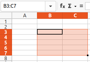
Similarly, a continuous cell block can be referenced by specifying the cell-id of the top-left corner cell of the block and the bottom-right corner cell of the block, separated by a colon (:). Example: B3:C7

So far we have used variable referencing which means that, if we simply copy paste the formula somewhere else, excel will study the pattern where it is placed and it will change the input data to the formula. To use absolute referencing, place a $ before the row-id and column-id of the cells. Example, $A$1. Now wherever we copy our formula, this cell referencing will be fixed.

We can even use mixed referencing where we permit excel to change only one of the two, either row or column. Example, $A1, C$5.

F4 is a useful shortcut to toggle between the type of cell referencing keeping the cell selected.

Cell Formatting

• Cell type can be many, string, number, float, date, time, etc.
• There are plenty of options from colouring or highlighting the cells to orienting the cell text along a direction and more.

• You can use format painter to copy the format of a cell and apply the same format over another cell

• You can use a cell as a column header and use it to filter the column data

Formulas

Useful formulas and their usage can be found in the this file.

Add checkbox: Developer tools -> Insert -> Form Controls -> checkboxes Format Control [if we want the checkbox to be tick or untick dependend on the boolean value of a cell]: Right click the checkbox and choose format control. -> Control tab

Add Radio Button: Developer tools -> Insert -> Form Controls -> Group Box Keeping the Group box selected, Developer tools -> Insert -> Form Controls -> radio button

To Protect Sheet: Review -> Protect Sheet

Data Validation Data Validation -> Setting -> List [for restricting entry from a particular group of cell]

VLOOKUP VLOOKUP ONLY works when search value is in the first column of the selected data. In the 4th argument of VLOOKUP, if we provide “false”, it will check for exact match. If we provide “true”, it will return partial match. The default is “true”. VLOOKUP will return false if the search value is not found in the first column of the selected data.

For searching from backwards or any arbitrary column, use a combination of the below two:

1. INDEX
2. MATCH

INDEX(A3:B7, MATCH(D7, B3:B7, 0), 1)

OR,

1. VLOOKUP
2. CHOOSE

VLOOKUP(E3, CHOOSE({1,2}, C3:C7, A3:A7), 2, false)

Here instead of choosing the entire data range, we select the two relevant columns (column where to look for match, and the column from which we will pick value). We then place these columns into proper order such that VLOOKUP gets the search column as the first column of the dataset generated by CHOOSE function. The indices {1,2} inside CHOOSE helps us to do this. Off course we can feed multiple columns in CHOOSE and arange the columns into a desired arrangement, but this can only be used inside some other formula or in a VBA code. It cannot be directly used in an Excel cell.

To substitute a text with another one: SUBSTITUTE(A15, “t”, “j”) # Replace all ‘t’ in the entry of cell A15 with ‘j’

VLOOKUP partial match: VLOOKUP(“*“&A15&”*”, D4:I13, false) # “*” is wildcard character and “&” concatenates the partial text of the input given in string cell A15

What to do in case of multiple matches:

• Make some unique column
• To find number of similar matches:
  • COUNTIF

ARRAY Formulas

• CSE formulas (Ctrl+Shift+Enter formulas) {=INDEX(A3:B7, MATCH(I4&I5, A3:A17&B3:B17, 0), 1)} # The “&” command concatenates the data blocks A3:A17 and B3:B17 in internal memory, which makes it different from other non-array like formulas. For this utility of INDEX CSE is required instead of just Enter.

HLOOKUP

Return row number of multiple instances of a match: Use the following 4 built in functions, IF SMALL ROW INDEX

We never discussed IF, SMALL and ROW functions before, so here we discuss a bit of these functions. SMALL function returns the kth smallest value of a selection of data. SMALL(A1:A20, 3) will return the 3rd smallest value of the data in cell range A1:A20. ROW gets the row number of a selection of cells. Thus ROW(2:2) // returns 2; ROW(E3) // returns 3; ROW(E4:G6) // returns {4,5,6}. IF is used to have an output based on logical operation. IF(C6>=70,”Pass”,”Fail”), IF(AND(A1>7,A1<10),”OK”,””), IF(OR(A1=”red”,A1=”blue”),B1+10,B1), IF(NOT(A1=”red”),B1+10,B1)

{SMALL(IF($A​$1:$F​$14=$A$16, ROW($A$1:$F$14)), ROW(1:1))} # Hit Ctrl+Shift+Enter [CSE]

ROW(1:1) when dragged, will increment to ROW(2:2) ROW(3:3) and so on.. Similarly we have COLUMN(A:A) will return 1, COLUMN(B:B) will return 2 and so on..

Troubleshooting: If we add or delete a column in a data set, our existing formulas which uses this data set will fail to work correctly. A trick is to build data for VLOOKUP dynamically as follows:

VLOOKUP(D8, A:C, MATCH(“HAIR”, 1:1, 0), FALSE) # Says to the VLOOKUP that return the column from the row of match, whose table header (identified by 1:1) has the string “HAIR”

Named Cells and Named Range: Static/Dynamic Static: Formulas -> Name Manager Dynamic named range: Formulas -> Name Manager Use OFFSET and COUNTA formula OFFSET function returns a reference to a range that is a specified number of rows and columns from a cell or range of cells, and COUNTA function returns the number of cells that are not empty in a range. OFFSET(‘Sheet_name’!$A​$1, 0, 0, COUNTA(‘Sheet_name’!​$A:$A), COUNTA(‘Sheet_name’!​$1:$1)) Leave Header on top of data range: OFFSET(‘Sheet_name’!$A$1, 0, 0, COUNTA(‘Sheet_name’!$A:$A)-1, COUNTA(‘Sheet_name’!​$1:$1))

Select anything Dynamically: Use OFFSET and COUNTA functions to first create a Dynamic named range, then use the name of this range in every formula that you use.

Creating a hyperlink (to another worksheet or a website or anything): Right click on the cell where you want to place the hyperlink, click ‘Hyperlink’. Choose from appropriate option

Return back from the hyperlink to the previous place: 1. Start recording a macro (Inside the Add-on name ‘Developer Tools’) 2. Click the hyperlink you created 3. Go back manually to where you came from (You can click undo) 4. Stop macro recording 5. To get to your macro, press Alt+F11 6. Look at the macro you created 7. Close the macro windows 8. Click Macro (In Developer Ribon) 9. Select the Macro name you saw in the window that you just closed, and press ‘Options’ 10. Add a Shortcut key for the macro 11. You may add a button and set button action as the macro

Conditional Formating (to know when the value is missing)

1. make a dynamic named array
2. to look up a cell and check whether the entry in the cell mathes with that of the created array list: MATCH(A7, mylist, 0)
3. To return a true or false value, put ISERROR before MATCH: ISERROR(MATCH(A7, mylist, 0))
4. Use this formulla in ‘new rule’ in ‘Conditional Formatting’ under Home ‘ribbon’

INDIRECT function: Redirects from cell A to cell B with the address given as string in cell A

Add Hyperlinks: For another sheet of the workbook:
=HYPERLINK(“#’Sheet2’!F15”, “Go there”) # Sheet2 being the name of the reference sheet to where you want to go. “Go there” is the friendly name of the cell where this formula is being used.

AND logical function: AND(E3=”Red”, E4=”Green”)

Select cells based on text, formulas, errors ets: Click on ‘Find and Select’ under ‘Home’ ribbon. Then click on ‘GoTo Special’.

Convert outputs of formulas to text data: Select the outputs Right click -> Copy Right click -> Paste Special (value)

Good Resources

https://analystcave.com/vba-cheat-sheet/