Mode Coupling Theory (MCT)- A short note
02 Aug 2021If you have never heard of Mode Coupling Theory (MCT), then well, from now on know this that, it is one of the fundamental theories that explains glass transition phenomena in simple liquids. In this write-up I will talk about what is this glass transition and how MCT helps in understanding it. I struggled to understand this theory for a considerable amount of time, and finally I managed to make some sense. Therefore, I will describe the birds eye view of the overall picture that I perceived. And just like the other posts on this site, I will keep the discussion succinct and to the point. So that I can recall the important aspects of it in future if I ever forget them. I will start out by making it very clear that by glass formation or glass transition, I am not specifically talking about the conventional glass that is widely used in our daily life (SiO2). Rather, it is the property and the arrival at this state which I will be discussing about. Even after so much of development on this field, there are still works going on to increase our knowledge on vitrification.
As a liquid is cooled down, it will eventually go bellow its freezing point when we hope that it will crystalline. The melting point becomes a material defining property. However, will the same thing happen if we cool the material rapidly? The short answer is no. The reason being, to arrive at a perfectly crystalline state, the material particles need to order themselves in an ordered lattice structure. However, if we cool rapidly from a disordered liquid state, the particles may not get time to relax and adjust themselves to the requirement of ordering. Upon quenching the liquid below a certain temperature, it enters into a super-cooled state where the viscosity increases by orders of magnitude and the flow of molecules stops for all practical timescales. This rapid cooling will not let the liquid molecules to “react” to the process of cooling and therefore they remain disordered in this new state too. Structural analysis shows that one can hardly distinguish between the the two state from their average microscopic arrangements.
Glass transition temperature (Tg) is this temperature at which if we suddenly cool a liquid, viscosity exceeds a value of 1012 Pa.s, or the structural relaxation time (τ) exceeds 100 s. The question that puzzled researchers were, how the viscosity (which is definitely related to some time scale of motion) show such dramatic change within the time of cooling without letting the average structure to change almost by any amount. Another interesting unknown quantity was the different timescale of motions associated with the phenomena of this glass transition. How are they related to the thermodynamic variables and what made them different for different particle size and composition. The answers to the above questions can be partially explained by MCT.
For the impatient ones: the MCT predicts the dynamic, given time-independent information as input [namely, static structure factor (S(k)) and bulk density $\rho$]. One needs to solve the MCT equation iteratively in order to get the solution under some assumption. (Why assumption? Well, as it will turn out that the exact MCT equation is impossible to solve otherwise!)
Let’s have some realisation through numbers and figures. A normal liquid has a viscosity of about 10-3 Pa.s, whereas the viscosity of a glassy solid is about 1012 Pa.s. The structure of the material in different phases is given in the following figure:
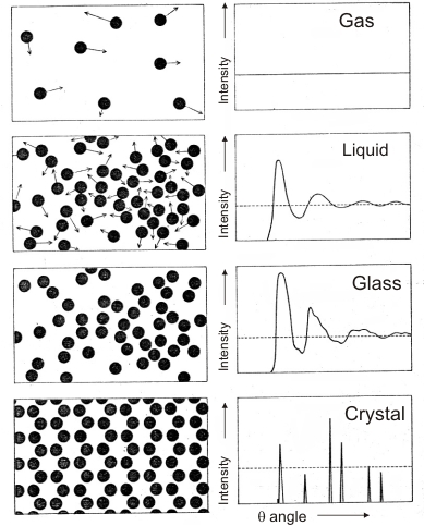
Notice how the liquid and glassy state look so similar in their ordering.
The time-dependent density correlation function F(k, t) is called intermediate scattering function. It captures the structure as well as dynamics. MCT let us envisage the behaviour and physical origin of this quantity through out its different relaxation processes. The static structure factor S(k) which can be obtained from a scattering experiment is equivalent to F(k, t=0). Here k is the wave-number ($k=2\pi / d$) which has a dimension of inverse length. In order to probe the relaxation dynamics at molecular scale, we choose k as approximately one inverse particle diameter.
Have a look at the typical plot of intermediate scattering function with time of a liquid plotted for $k=2\pi$ (i.e $d=1$):

As the system is cooled, the overall relaxation time increases very rapidly and this happens in steps. At short time, the particles undergo ballistic motion. Here they take short linear moves without colliding with neighbours. Occasionally, these particles may take a random path within the “cage” of its neighbours, which is called by $\beta$ relaxation. On an even longer time-scale, particles may move out of this cage which is associated to another kind of relaxation process called $\alpha$ relaxation.
In case of glassy solid, the onset time of $\alpha$ relaxation relaxation is very long and the curve appears to remain constant for a relevant macroscopic time-scale. Without any $\alpha$ relaxation tail.
Steps to derive the MCT equation:
-
We start with writing a correlation matrix of spatial density ($\rho(\textbf{k}, t)$) and current density modes ($j(\textbf{k}, t)$) ( time derivative of spatial density): \(C_{\alpha \beta} = \left < A_{\alpha}(0)|A_{\beta}(t)\right >\) $ where $ \(A = \begin{pmatrix} \rho(\textbf{k}, t)\\ j(\textbf{k}, t) \end{pmatrix}\)
-
Using C and A we define a projection operator $P_A$
\(P_A = \sum_{\alpha, \beta} |A_{\alpha}> [C(0)]^{-1}_{\alpha \beta} <A_{\beta}|\) This projection operator is constructed in such a way so that $P_A X$ will project X onto A(0)
-
With the above two, we can write equation of the classical function of phase space variable A.
$A(t) = e^{iLt}A(0)$
where L is the Louisville’s operator.
A differentiation in time would give: $\frac{dA(t)}{dt}=e^{iLt}iLA(0)$
-
We break the motion of X into two subspace: one in the subspace of A(0)-often referred as “slow” component, and another orthogonal to A(0).
Using the projection operator $P_A$ and its complement $1 - P_A$, this becomes possible.
-
We insert ($P_A + 1 - P_A$) in between:
$\frac{dA(t)}{dt}=e^{iLt} [P_A + (1 - P_A)] iLA(0)$
which upon following some fancy mathematical steps (For an elaborate calculation, look for David Reichman), lands up to the exact MCT equation:
-
\[\frac{dA(t)}{dt} = i \Omega \cdot A(t) - \int_0^{t} d\tau K(\tau) \cdot A(t-\tau) + f(t)\]
where \(i\Omega = \left < A(0)^{*}|iLA(0) \right > \cdot \left < A(0)^{*}|A(0) \right >^{-1}\)
\(K(t) = \left < f(0)^{*}|f \right > \cdot \left < A(0)^{*}|A(0) \right >^{-1}\) and \(f(t) = e^{i(1-P_A)Lt} i (1-P_A) LA(0)\) $\Omega$ is called the frequency matrix
f(t) is called the fluctuating force
- For the correlation matrix C, this equation will take the exact form leaving the fluctuating force term: \(\frac{dC(t)}{dt} = i \Omega \cdot C(t) - \int_0^{t} d\tau K(\tau) \cdot C(t-\tau)\) with the same form of frequency matrix and fluctuating force term.
For the time being it suffices to know that:
-
f(t) is orthogonal to A(0), as f(t) contains the complementary projection operator $(1-P_A)$.
- The memory function K(t) is given by the time-auto-correlation function of the fluctuating force f(t).
- “K(t) and f (t) embody how our slow variable A–which at time t = 0 lives strictly in the slow subspace–will gradually evolve under the influence of the rest of the universe”
- Equation 4 and 8 are called Generalized Langevin Equation.
- Till this far, every thing is exact and it is impossible to go any further without some approximations.
Approximations
-
Representing K(t) as a four-point density correlation function: \(K(t) ~ \sum_{\textbf{k}_1, \textbf{k}_2, \textbf{k}_3, \textbf{k}_4} <\rho^*(\textbf{k}_1, 0) \rho^*(\textbf{k}_2, 0) e^{i[1-P_A]Lt} \rho(\textbf{k}_3, 0)\rho(\textbf{k}_4, 0)>\)
-
Factorise four-point correlation functions as a product of two two-point correlation functions and replace $e^{i[1-P_A]Lt}$ with $e^{iLt}$ \(K(t) ~ \sum_{\textbf{k}_1, \textbf{k}_2, \textbf{k}_3, \textbf{k}_4} <\rho^*(\textbf{k}_1, 0) \rho(\textbf{k}_1, t) e^{iLt} \rho^*(\textbf{k}_2, 0)\rho(\textbf{k}_2, t)>\) This approximation is made without solid reasoning; rather just to make more simplification.
If we allow these approximations then we can arrive at the full MCT equation (by equating the lower-left side of the matrix equation):
\[\frac{d^2F(k,t)}{dt^2} + \frac{k_BTk^2}{mS(k)}F(k,t) + \int_0^t ds K_{MCT} \frac{dF(k, t-s)}{dt} = 0\]with the memory function as,
\[K_{MCT}(k,t) = \frac{\rho k_B T}{16 \pi^3 m} \int d\textbf{q} |V_{\textbf{q, k-q}}|^2 F(q,t) F(|\textbf{k-q}|,t)\]with
\[V_{\textbf{q, k-q}} = k^{-1} [(\textbf{k.q}) c(q) + \textbf{k}\cdot (\textbf{k-q}) c(|\textbf{k-q}|)]\]which is referred as vertices with $c(k) = \rho^{-1}[1-1/S(k)]$
Here, $k_B$ is the Boltzmann constant, $m$ is the particle mass, $\rho$ is the bulk density
Equation 11 can be solved just like any other self-consistent equation with the boundary condition being:
$F(k, 0)/S(k) = 1$ and $\dot{F}(k, 0) = 0$
For numerical solution scheme, you may check out Elijah Flenner and Grzegorz Szamel PRE (2005).
Okay, so now that we know that this can be solved, I will now point out the essence of the terminologies that were used in the formulation:
Comparing MCT equation with one-dimensional damped harmonic oscillator:
$x(t) = F(k,t)$
$\Omega_{21} = \omega^{2} = \frac{k_BTk^2}{mS(k)}$
$K_{MCT} = ax^2(t)$ , where a is a damping factor (represents the effective strength of vertices at a temperature)
where the one-dimensional damped harmonic oscillator has the form: \(\ddot{x}(t) + \omega^{2}x(t) + \int_{0}^{t} K_{MCT}(s) \dot{x}(t-s) ds = 0\)
I believe that the above comparison was sufficient enough to justify the names given to $\Omega$ and $K(t)$
Equation 12 is called schematic MCT model.
Substituting $K_{MCT} = a \delta$ the schematic MCT equation becomes identical to our most familiar damped harmonic oscillator.
However, as we will see that the quadratic form of $K_{MCT} = ax^2(t)$ , is what makes MCT successful in treating liquid glass transition.
Equation 12 can be solved with the quadratic form of $K_{MCT} = ax^2(t)$ in an iterative self-consistent way and the results show strong feedback mechanism depending on “a” that drives the transition.
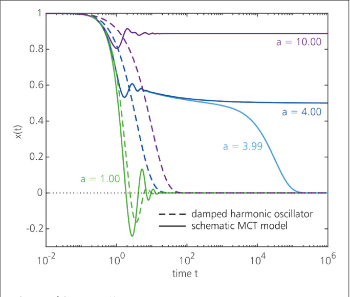
As “a” increases, x(t) seizes to drop any sooner. And beyond the critical value of $a=4$, it stays constant for all practical purposes.
Thus, a non-linear dynamical feedback mechanism through the memory function decides the glass transition and dynamics.
For solving the full wavevector-dependent MCT equation, one can guess an initial guess of F(k,t) for all relevant k, and solve it individually using self-consistent method
For systems undergoing Brownian Dynamics instead of Newtonian Dynamics, Liouvillian operator should be replaced with Smoluchowski operator. In this case, $k_B T$ is replaced with the diffusion constant D.
From MCT we can predict that close to the glass transition temperature $T_c$, the relaxation time of F(k, t) diverges as a power law, $\tau \sim (T-T_c)^{\gamma}$.
MCT also predicts that power law of $\beta$ relaxation and $\alpha$ relaxation
Close to $T_c$, the MCT exponents are related as \(\frac{\Gamma(1-a)^2}{\Gamma(1-2a)} = \frac{\Gamma(1+b)^2}{\Gamma(1+2b)}\) where $\Gamma$ is the Gamma function.
During $\alpha$ relaxation, the final decay of F(k, t) has the functional form of $e^{(\frac{-t}{\tau})^{\beta}}$. Where $\beta$ is a value between 0 and 1 (inclusive). Known as Kohlrausch (stretched exponential) behavior.
The variation of $\tau_{\alpha}$ with temperature (T) shows two kinds of dependence for two group of glass forming liquids. The kind which shows Arrhenius temperature dependence with $T$ is fitted with the functional form: \(\tau_{\alpha} = \tau_0 e^{\frac{E_a}{k_B T}}\) is called “Strong liquids”
The other kind of temperature dependence which is fitted with the form: \(\tau_{\alpha} = \tau_0 e^{\frac{E_a}{k_B (T-T_0)}}\)
is called “fragile liquid” and designated as Vogel–Fulcher–Tammann (VFT) temperature dependence.
$E_a$ is the activation energy which is a measure of the fragility [the degree to which the relaxation time increases as $T_g$ (the experimental glass transition temperature) is approached]
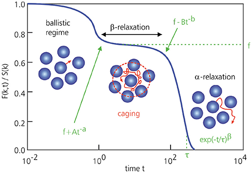
The figure above shows the relevant regions along with the predictions of MCT.
A naive C++ and python implementation to solve the schematic MCT model is given below:
#include <bits/stdc++.h>
#include <iostream>
#include <stdlib.h>
#include <math.h>
#include <fstream>
#include <sstream>

#define iter 1000000
#define del_t 0.0001

using namespace std;
using std::ifstream;

int main()
{

int i,j ;
double x[iter]={0};
double v[iter]={0};
double omega = 1 ;
double A = 1 ;
double a ;
double Int ;


ofstream F_file;
string filename2;
filename2 = "output.txt";
F_file.open(filename2.c_str(), ios::out);

x[0] = 1 ;
v[0] = 0 ;

for(i=0;i<iter;i++){

	x[i+1] = x[i] + v[i] * del_t ;

        Int = 0 ;

        for( j = 0 ; j < i; j++ )
        {
        	Int = Int + x[j] * x[j] * v[i-j] * del_t ;
        }

        a = -omega * omega * x[i] - A * Int ;

	v[i+1] = v[i] + a * del_t ;

	F_file << i * del_t << "   " << x[i] << endl ;

}

F_file.close();

return 0;

}
import matplotlib.pyplot as plt
# List Implementation:

itterations = 1000000
delta_t = 0.0001
omega = 1
a = 5

x = [1]
v = [0]
time = [0]

for i in range(0, itterations):
    x.append(x[i] + v[i]*delta_t)

    Int = 0.0
    for j in range(0, i):
        Int = Int + x[j]*x[j]*v[i - j]*delta_t

    v.append(v[i]+ (-omega * omega * x[i] - a * Int) * delta_t)
    time.append(i * delta_t)

    #print(i*delta_t, x[i-1])

plt.plot(time, x)
plt.show()
This write-up was meant to provide a rough idea of the concept, and also compiled with the intent of brushing up the concept in any future time. For an even more in-depth view of MCT, please refer to the following articles:
- Janssen, Liesbeth. “Mode-coupling theory of the glass transition: A primer.” Frontiers in Physics 6 (2018): 97.
- Reichman, David R., and Patrick Charbonneau. “Mode-coupling theory.” Journal of Statistical Mechanics: Theory and Experiment 2005.05 (2005): P05013.
- Flenner, Elijah, and Grzegorz Szamel. “Relaxation in a glassy binary mixture: Comparison of the mode-coupling theory to a Brownian dynamics simulation.” Physical Review E 72.3 (2005): 031508.
- Debenedetti, Pablo G., and Frank H. Stillinger. “Supercooled liquids and the glass transition.” Nature 410.6825 (2001): 259-267.
- Swenson, Jan, and Silvina Cerveny. “Dynamics of deeply supercooled interfacial water.” Journal of Physics: Condensed Matter 27.3 (2014): 033102.